Image Generation and Manipulation Overview
A wide range of tools are available for generating and manipulation images programmatically.
Where this is done in situ, the local context should help the relationship between text and image to remain consistent.
Generating Images
One of the advantages of generating diagrams from scripts is that it can make them easier to maintain.
Creating SVG Images
Various tools exist that support the creation of SVG images from high level diagramming packages. We can also create SVG images at a lower, directly scripted level:
%%capture
try:
    import drawSvg
except:
    %pip install drawSvg
import drawSvg as draw

d = draw.Drawing(200, 100, origin='center', displayInline=False)

# Draw an irregular polygon
d.append(draw.Lines(-80, -45,
                    70, -49,
                    95, 49,
                    -90, 40,
                    close=False,
            fill='#eeee00',
            stroke='black'))

# Draw a rectangle
r = draw.Rectangle(-80,0,40,50, fill='#1248ff')
r.appendTitle("Our first rectangle")  # Add a tooltip
d.append(r)

# Image size
#d.setPixelScale(2)  # Set number of pixels per geometry unit
d.setRenderSize(200,200)  # Alternative to setPixelScale

# Save image to file
#d.saveSvg('example.svg')
#d.savePng('example.png')


d  # Display as SVG

#d.rasterize()  # Display as PNG

Manipulating Images
skimage
The skimage (scikit-image) Python package provides a wide range of image processing tools.
Colour separation
#Example from http://scikit-image.org/docs/dev/auto_examples/color_exposure/plot_ihc_color_separation.html
import numpy as np
import matplotlib.pyplot as plt
from skimage import data
from skimage.color import rgb2hed, hed2rgb
# Example IHC image
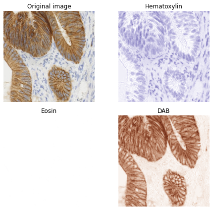
ihc_rgb = data.immunohistochemistry()
# Separate the stains from the IHC image
ihc_hed = rgb2hed(ihc_rgb)
# Create an RGB image for each of the stains
null = np.zeros_like(ihc_hed[:, :, 0])
ihc_h = hed2rgb(np.stack((ihc_hed[:, :, 0], null, null), axis=-1))
ihc_e = hed2rgb(np.stack((null, ihc_hed[:, :, 1], null), axis=-1))
ihc_d = hed2rgb(np.stack((null, null, ihc_hed[:, :, 2]), axis=-1))
# Display
fig, axes = plt.subplots(2, 2, figsize=(7, 6), sharex=True, sharey=True)
ax = axes.ravel()
ax[0].imshow(ihc_rgb)
ax[0].set_title("Original image")
ax[1].imshow(ihc_h)
ax[1].set_title("Hematoxylin")
ax[2].imshow(ihc_e)
ax[2].set_title("Eosin") # Note that there is no Eosin stain in this image
ax[3].imshow(ihc_d)
ax[3].set_title("DAB")
for a in ax.ravel():
a.axis('off')
fig.tight_layout()
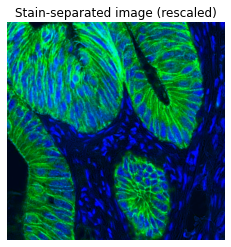
from skimage.exposure import rescale_intensity

# Rescale hematoxylin and DAB channels and give them a fluorescence look
h = rescale_intensity(ihc_hed[:, :, 0], out_range=(0, 1),
                      in_range=(0, np.percentile(ihc_hed[:, :, 0], 99)))
d = rescale_intensity(ihc_hed[:, :, 2], out_range=(0, 1),
                      in_range=(0, np.percentile(ihc_hed[:, :, 2], 99)))

# Cast the two channels into an RGB image, as the blue and green channels
# respectively
zdh = np.dstack((null, d, h))

fig = plt.figure()
axis = plt.subplot(1, 1, 1, sharex=ax[0], sharey=ax[0])
axis.imshow(zdh)
axis.set_title('Stain-separated image (rescaled)')
axis.axis('off')
plt.show()
import numpy as np
from skimage.data import camera
from skimage.filters import roberts, sobel, scharr, prewitt
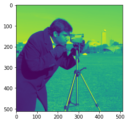
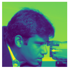
image = camera()
plt.imshow(image);
#What is the size of the image in x/y pixels?
image.shape

#We can zoom in to a part of the image
cropped_image = image[50:200, 150:300]
plt.axis('off')
plt.imshow(cropped_image);
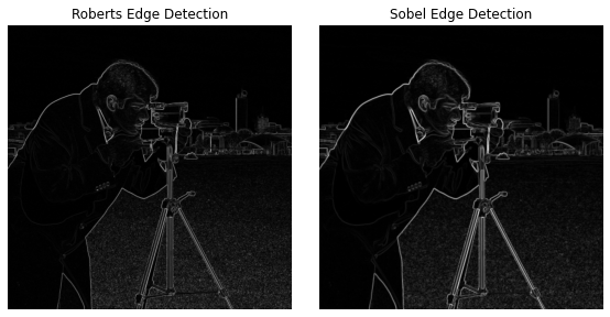
A wide range of filtering opportunities exist. For example, edge detection:
#http://scikit-image.org/docs/dev/auto_examples/edges/plot_edge_filter.html

edge_roberts = roberts(image)
edge_sobel = sobel(image)

fig, ax = plt.subplots(ncols=2, sharex=True, sharey=True,
                       figsize=(8, 4))

ax[0].imshow(edge_roberts, cmap=plt.cm.gray)
ax[0].set_title('Roberts Edge Detection')

ax[1].imshow(edge_sobel, cmap=plt.cm.gray)
ax[1].set_title('Sobel Edge Detection')

for a in ax:
    a.axis('off')

plt.tight_layout()
plt.show()

#Other sets of image processing examples to try:
#https://auth0.com/blog/image-processing-in-python-with-pillow/
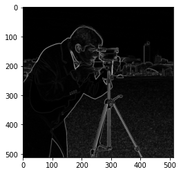
OpenCV
The OpenCV package is a very powerfl image processing toolkit.
import cv2

ddepth = cv2.CV_64F  # 64-bit float output
#Do filter in x and y directions
sobelx = cv2.Sobel(image, cv2.CV_64F, 1, 0)
sobely = cv2.Sobel(image, cv2.CV_64F, 0, 1)
sobel = cv2.sqrt(cv2.addWeighted(cv2.pow(sobelx, 2.0), 1.0, cv2.pow(sobely, 2.0), 1.0, 0.0))

plt.imshow(sobel, cmap='gray');
#https://www.pyimagesearch.com/2014/01/22/clever-girl-a-guide-to-utilizing-color-histograms-for-computer-vision-and-image-search-engines/
import cv2
def colHistRGB(image):
    # grab the image channels, initialize the tuple of colors,
    # the figure and the flattened feature vector
    chans = cv2.split(image)
    #is this right? Opencv seems to mess with RGB/BGR and I have no idea what colour is what...
    colors = ("b", "g", "r")
    plt.figure()
    plt.title("'Flattened' Color Histogram")
    plt.xlabel("Bins")
    plt.ylabel("# of Pixels")
    features = []

    #What do the bins represent? Value of colour channel?
    # loop over the image channels
    for (chan, color) in zip(chans, colors):
        # create a histogram for the current channel and
        # concatenate the resulting histograms for each
        # channel
        hist = cv2.calcHist([chan], [0], None, [256], [0, 256])
        features.extend(hist)

        # plot the histogram
        plt.plot(hist, color = color)
        plt.xlim([0, 256])
Consider the following image:
from matplotlib.pyplot import imread

##Image from https://www.open.edu/openlearn/history-the-arts/making-sense-art-history/content-section-5.6
orange_image_file = 'plate10.jpg'

orange_image = imread(orange_image_file)

plt.imshow(orange_image);
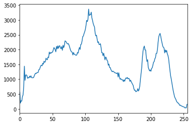
We can look at a colour histogram:
colHistRGB(orange_image)
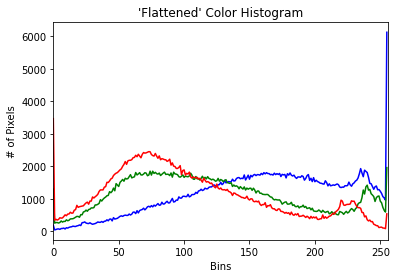
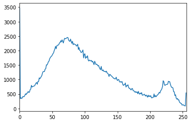
One possible problem with the chart is that we don’t know whether the separate high RGB channel values are at the same pixel (eg a white pixel) or spread across pixels.
Mayb a gray level brightness would identify high average RGB values as “bright” pixels?
from skimage.io import imsave

imsave('testout.png', orange_image)
#COLOR_BGR2GRAY COLOR_RGBA2BGRA
img = cv2.imread('testout.png',cv2.COLOR_BGR2GRAY)
hist = cv2.calcHist([img],[0],None,[256],[0,256])
plt.plot(hist)
plt.xlim([0, 256])

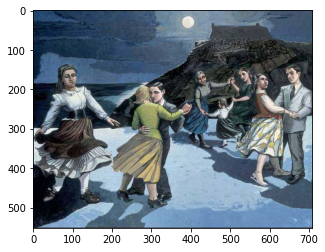
How about a blue themed image - can we learn anything from the RGB plot about that?
#Image from https://www.open.edu/openlearn/history-the-arts/making-sense-art-history/content-section-5.6
blue_image_file = 'plate14.jpg'

blue_image = imread(blue_image_file)

plt.imshow(blue_image);
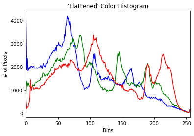
Here’s the colour histogram:
colHistRGB(blue_image)
And the greyscale brightness:
imsave('testout2.png', blue_image)

img = cv2.imread('testout2.png',cv2.COLOR_BGR2GRAY)
hist = cv2.calcHist([img],[0], None, [256],[0,256])
plt.plot(hist)
plt.xlim([0, 256])