Statistics in R
The code that can be executed in Jupyter notebook code cells is determined by the Jupyter kernel with which the notebook is associated and against which it is run.
For the author, this means that a single authoring environment, such as the classic Jupyter notebook interface, can be used to author documents whose outputs may be generated from a wide range of programming languages.
Note
Typically, all the code cells will be run against a single language kernel.
However, various workarounds are possible that support polyglot notebooks that allow multiple languages to be used across different cells.
This notebook, for example, is associated with an R kernel rather than a Python kernel.
An Example in R
The following code cell shows how we can load in an R library to a native R environment:
library(ggplot2)
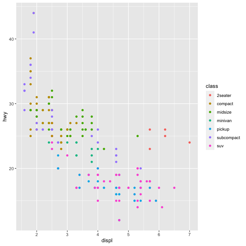
And then render a rich output from it:
ggplot(mpg, aes(displ, hwy, colour = class)) +
  geom_point()
Symbolic Computation in R
We can use the Ryacas package to provide us with a symbolic computational environment based on Yacas, although inlining items using glue is not possible because we aren’t working in a Python environment.
Note
The R knitr/bookdown workflow currently provides a much simpler route to producing texts with inlined code output.
library(Ryacas)
Create some objects and a function around them:
x <- ysym("x")
y <- ysym("y")

f <- (1 - x)^2 + 100*(y - x^2)^2
And render the function as LaTeX:
library('IRdisplay')

display_latex(paste('$$', tex(f), '$$', sep=''))
We can evaluate the function by casting the symbolic expression to R and setting the variables:
eval(as_r(f), list(x = 2, y = 2))
Do some sums, such as find the derivative with respect to \(x\), or \(y\):
Latex = function(s){
        display_latex(paste('$$', tex(s), '$$', sep=''))
}

g <- deriv(f, c("x", "y"))
Latex(g)
We can assign values into the expression:
yac_assign(3, "x")

Latex(f)
And reset the symbolic variable:
yac_silent("Clear(x)")

Latex(f)