Maths Overview
Trivially, notebooks provide us with a simple editing environment for combining markdown text, simple inline LaTeX and LateX blocks, and code cells prefixed with the %%latex block cell magic.
This also us to notebooks a medium for creating content blends narrative text with mathematical notation.
Note
Within a notebook user interface, native support for LaTeX inline in markdown cells is limited to that subset of LaTeX that can be parsed by the MathJax parser.
LaTeX parsing magics and code output transclusion can be used to provide access to a full featured LaTeX parser.
In addition, code cells allow us to perform mathematical computations and generate graphical outputs.
In a complete one piece generative document flow publishing system where we guarantee the correctness of calculations and formal arguments, as wel as the correctness of output graphics in relation to the body of the content, we ideally need to find a way to relate the (symobolic) mathematical content to the code that is executed.
Using a symbolic maths package such as sympy, we can create symbolic computational expressions that can be used to calculate (compute) expressions at a symbolic level as well as rendering those expressions in mathematical form using LaTeX (Mathjax). For rendering integrated one piece content in Jupyter book, the Python myst_nb.glue() provides a means for inline code outputs, but this requires a Python kernel. For bookdown workflows, outputs from all supported languages can be inlined [ TO DO — CHECK ].
If tight integration with the text is not required, or if markdown output can be generated from code, computation using a wide range of other languages can is enabled by installing the appropriate Jupyter kernel (curated list of Jupyter kernels). For example, several kernels are available that are particularly suited to a range of mathematics related activities such as statistical computing, symbolic maths and numerical computation. For example:
Rstatistical computing and graphics;Statastatistical computing;SageMathcomputer algebra system;Maximacomputer algebra system;Octavenumerical computation;SciLabnumerical computation;Matlab mathematical computing;
Wolfram Language mathematical computing;
Gnuplotcharts.
Note
We can also write markdown in a code cell by converting to the code cell to a de facto markdown cell using the %%markdown block magic.
Rendering equations Using MathJax
Equations can be rendered as a block using MathJax in a markdown cell.
See this third party Typesetting Equations demonstration notebook for further examples.
MathJax content can also be rendered inline. For example, we can include the expression \(\sqrt{3x-1}+(1+x^2)\) embedded within a line of text.
Rendering equations from sympy
Guaranteeing the truth of a derived mathematical expression is often difficult if multiple steps of working are required and is further complicated particulalry if the expression is a complicated one.
Using a symbolic maths package such as sympy allows derived expressions to be generated automatically and then embedded into book output.
The following example is taken from “Technical writing: using math”, Nicolás Guarín-Zapata.
Given the expression:
from sympy import symbols, exp, sin

x = symbols("x")

f = exp(-x**2)*sin(3*x)
f
we can find its second derivative as:
from sympy import diff

fxx = diff(f, x, 2)
fxx
Since the second derivative is calculated, and the equation is then rendered to a LaTeX form automatically, we know that the expression is correct (although it may not be in the form we require).
Rendering Matrices
If we have a numpy array, we can render it as a LaTeX styled matrix using a Python package such as numpyarray_to_latex.
For example, here’s a random 4 x 5 array with round brackets (the default, although other bracket styles are customisable):
#https://github.com/benmaier/numpyarray_to_latex
#%pip install --upgrade numpyarray_to_latex
import numpy as np
from numpyarray_to_latex.jupyter import to_jup

array = np.random.randn(4,5)

to_jup(array)
We can access the raw LaTeX if required:
from numpyarray_to_latex import to_ltx

latex_txt = to_ltx(array)
print(latex_txt)
\left(
\begin{array}{}
 -0.8542 & -0.3806 &  1.4083 &  0.6391 &  0.4946\\
  0.2284 &  0.0386 & -0.5367 &  0.2094 & -1.5896\\
 -0.5615 & -0.0187 & -1.0757 & -0.7719 & -0.4398\\
 -1.2401 &  0.4120 &  1.3512 & -0.2385 &  0.2908
\end{array}
\right)
Matrices can also be rendered via sympy (using square brackets), as can the results of matrix calculations. For example, let’s cast the above array as a sympy.Matrix and add it to itself:
from sympy import Matrix

Matrix(array) + Matrix(array)
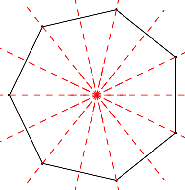
Embedding LaTex / TikZ Graphical Outputs
We can use the ipython_magic_tikz magic to provide access to a TikZ/LaTeX parser to allow us to generate diagrams from TikZ) scripts.
#%pip install git+https://github.com/innovationOUtside/ipython_magic_tikz.git
%load_ext tikz_magic
%%tikz
\usetikzlibrary{shapes.geometric, calc}
\def\numsides{7} % regular polygon sides
\node (a)
[draw,  blue!0!black,rotate=90,minimum size=3cm,regular polygon, regular polygon sides=\numsides] at (0, 0) {};

\foreach \x in {1,2,...,\numsides}
  \fill (a.corner \x) circle[radius=.5pt];

\foreach \x in {1,2,...,\numsides}{
  \draw [red,dashed, shorten <=-0.5cm,shorten >=-0.5cm](a.center) -- (a.side \x);
  \draw [red,dashed, shorten <=-0.5cm,shorten >=-0.5cm](a.center) -- (a.corner \x);}